How To Draw Bar Graph On Excel
How To Draw Bar Graph On Excel - Web create a bar chart. You can draw them by hand. For data with a single value to each variable, excel usually uses the name of the dependent variable as the chart title. Resize the chart for better readability. Modify chart by sorting column data. Select insert > recommended charts. A visual element called an error bar is used to display the variability or uncertainty in a set of data. Go to the insert tab. Web first, select the data and click the quick analysis tool at the right end of the selected area. Web once you have highlighted your data, you can insert a bar graph by clicking on the “insert” tab in the excel ribbon. Web create a bar chart. Web creating a bar graph in excel involves setting up the data, selecting the data, inserting the graph, customizing it, and adding labels and a legend. A visual element called an error bar is used to display the variability or uncertainty in a set of data. Secondly, from the insert tab >>> insert column or. Now, you will find an icon for creating a stacked bar, a 100% stacked bar, a 3d stacked bar, and a 100% 3d. In this tutorial, you will learn how to make a bar graph in excel and have values sorted automatically descending or ascending, how to create a bar chart in excel with negative values, how to change the. Select all the data that you want included in the bar chart. You have reached the end of this page. Make a percentage vertical bar graph in excel using clustered column. Select insert > recommended charts. Bar charts are used to graphically represent categorical data or to track changes over time or show differences in size, volume, or amount. If you want different labels, type them in the appropriate header cells. This wikihow article will teach you how to make a bar graph of your data in microsoft excel. 958k views 4 years ago 1 product. A bar graph is not only quick to see and understand, but it's also more engaging than a list of numbers. Be sure to include the column and row headers, which will become the labels in the bar chart. Select the clustered column option from the chart option. Web adding axis title. Click the bar chart icon. Create a chart from start to finish. The chart will appear in the same worksheet as your source data. Create pie, bar, and line charts. Once your data is selected, click insert > insert column or bar chart. Web the steps used to create a bar chart in excel are as follows: You can select the data you want in the chart and press alt + f1 to create a chart immediately, but it might not be the best chart for the data. Web first, select the data and click the quick analysis tool at the right end of the selected area. The chart design tab is created.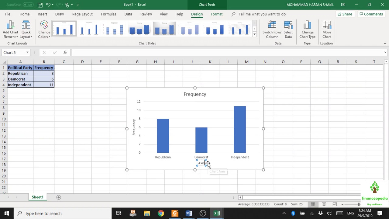
How to draw a bar chart in Excel? YouTube
How To Make A Multiple Bar Graph In Excel YouTube
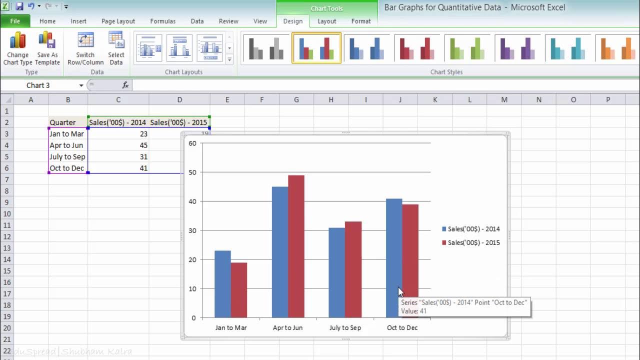
Simple Bar Graph and Multiple Bar Graph using MS Excel (For
To Create A Bar Chart, Execute The Following Steps.
Web Once You Have Highlighted Your Data, You Can Insert A Bar Graph By Clicking On The “Insert” Tab In The Excel Ribbon.
Web Create A Bar Chart.
Resize The Chart For Better Readability.
Related Post: